by Rudolph Kalveks
Scarcely a day goes by without a new and apparently contradictory announcement by some epidemiologist regarding the outlook for the COVID-19 coronavirus (“Coronavirus”). But what lies behind their models and to what extent should their pronouncements be taken at face value?
It is well known to all experienced data analysts, whether in science or in economics, that given a sufficient number of model parameters to play with, one can achieve a spectacular fit to historic data, only to find that model projections bear no relation to subsequent events.
The philosopher of science, Willard Van Orman Quine, coined the phrase “Underdetermination of Theory”, which applies in the situation where different theories are consistent with the same body of evidence. Models are inherently underdetermined and it is easy for their assumptions to take on a life of their own and to start predicting phenomena that are pure model artefacts rather than being representative of the physical system being studied. Given observational data in science, great care needs to be taken to distinguish the signal from the noise. This is easiest when there are prior grounds for expecting a certain type of signal and when the signal can be described with a few parameters. Gravitational physicists working with the LIGO interferometer apply such principles when detecting gravitational waves from merging black holes.
So, let us hunt for the signal in the Coronavirus data. What signal does the data contain? In particular, what does it suggest about the progress of the epidemic and whether a second wave could reasonably be expected? In an ideal world, epidemiologists would have extensive and accurate data on individual cases, their progress and recovery. Unfortunately, in the real world, different countries classify cases and deaths according to different criteria, and, moreover, change their classifications over time. For example, increases in the level of testing have the effect of increasing the cases recorded, but with no change in the underlying state of the population. And although organisations such as Worldometer make efforts to ensure data integrity, some data noise remains, for example, from the vagaries of daily recording systems in reporting countries. For such reasons, the approach taken in this signal tracing exercise has been to work with the cumulative country daily death statistics reported by Worldometer. If we make the assumption that deaths are in a broadly constant ratio to recoveries, these become the “canaries in the mine” that can tell us about the prevalence and progress of the infection in the wider population.
Epidemiology has a standard tool, the Susceptible–Infected–Recovered/Resolved or (“SIR”) model. In its simplest form, this decodes an epidemic in terms of transfers between three sub-populations – those susceptible to infection, those infected (and generally infectious), and those recovered or deceased (and in either case no longer infectious). The population at large is not necessarily susceptible; some may have natural or acquired immunity, for example by vaccination; others may be effectively isolated.
The dynamics of epidemiology interpret the rate of new infections as the product of the number of infectious individuals, times the proportion of susceptible targets, times some parameter (say, alpha). This is similar to the velocity of a chemical reaction, where the rate is proportional to the concentrations of the reagents. Alpha is inversely proportional to the period over which an epidemic doubles in its early stages. The rate of recovery of infected individuals is governed by a second parameter (say, beta). Beta is inversely proportional to the median time taken for recovery. This is similar to a half-life observed in radioactive decay. The ratio alpha:beta is often termed R0, and an epidemic can only start if this is greater than unity.
Over time, the rate of new infections declines, as the number of susceptible individuals is reduced. Consequently, R0 declines to a lower value R. Eventually R falls below unity and the number of infected cases starts to decline. Importantly, the magnitude of R0 influences the penetration of an epidemic. With a value of R0 only slightly above unity, an epidemic soon fizzles out; on the other hand, with a high value of R0, an epidemic may penetrate an entire susceptible population.
These relationships can be formalised in a few simple equations. Once the parameters alpha and beta are set, the course of an epidemic can be modeled through to its finish, starting from the day that patient zero is introduced to a susceptible population.
Of course, real epidemics are not quite so simple. Populations are not homogeneous, being neither equally susceptible (clinically) nor equally accessible (by proximity). Government social measures, medical treatments and other factors may cause the parameters alpha and beta to change over time, or may isolate a proportion of the susceptible population for a period. There may be a lag between acquiring an infection and becoming infectious. All these factors introduce potential complexities – more sub-populations, more parameters, and so on. But there are only so many independent data points available to tutor the assumptions used to model an epidemic’s dynamics.
To identify the signal from a chosen regional population, we assume the basic SIR model and ask what parameters lead to the best fit to the cumulative daily death statistics, using the least squares method for minimising errors. In addition to alpha and beta, the tuneable parameters include the date at which patient zero is introduced to a susceptible population and its size (say, gamma). Mathematically speaking, a straight line is described by two parameters, its gradient and intercept, while a curve with two independent curvature features, such as growth and decay, requires at least two more. So, with a total of four parameters, this is a minimal SIR model.
In physics, a theory that is known to be oversimplified, but nonetheless provides a good fit to the data and makes useful predictions is often termed an “effective theory”.
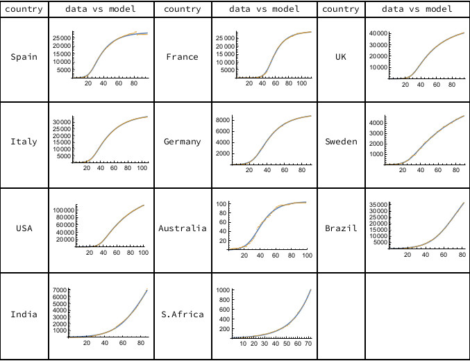
Intriguingly, we find that this minimal SIR model gives a good fit to the data for a sample of countries, as shown in Figure 1. All the models account for over 99% of the variance in the historic data. Having found the parameters for our country models, we can ask what they tell us about the dynamics and progress of the epidemic.
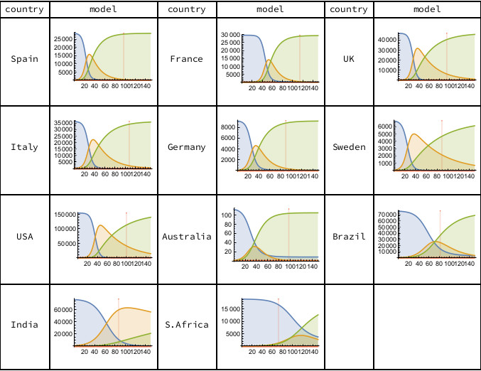
Figure 2 shows the progress between the three SIR model sub-populations. In most countries, the Susceptible (blue) sub-populations have very largely become either Infectious (orange) or Resolved (green). The epidemics in the European countries, the USA and Australia are currently the furthest advanced (as determined by the ratio of Resolved to Infected). In Brazil, India and South Africa the epidemic is still in its growth phase, with no sign of a curvature inflection in the time series of cumulative deaths.

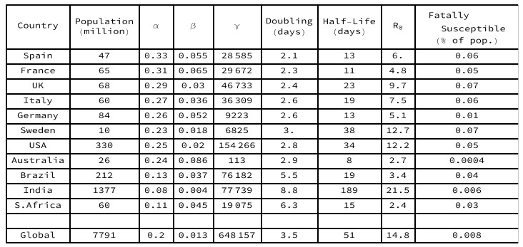
Doubling days = natural log(2) / alpha. Half-life = natural log(2) / beta. R0=alpha/beta.
Gamma = potentially fatally susceptible population.
Key statistics for each of these selected country models are set out in Table 1. The European countries have parameters with a similar order of magnitude, namely initial doubling between 2 and 3 days, and infectious half-lives between 11 and 23 days (with the exception of Sweden). The modelled R0 values are all far above unity, accounting for the rapid initial penetration of the susceptible populations observed in Figure 2. In Sweden and in the USA, the epidemics are not yet as far into the decay phase, so their long recovery half-lives may be overestimates. In Australia, the low penetration of the entire population and the persistence of a susceptible yet uninfected sub-population, reflects success in isolating large regions of the country. In Brazil, India and South Africa, the doubling period is markedly longer than in the European countries, accounting for the slow rate of spread, so the epidemic is still at an early stage after many days.
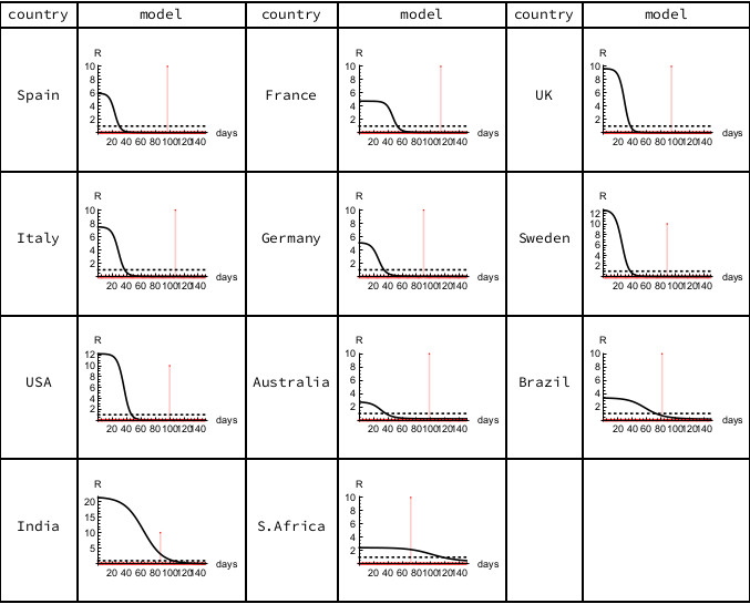
The modeled epidemiological R declines continuously from its initial value R0 as each epidemic progresses, with the peak of the Infectious sub-population occurring when the epidemiological R equals unity. For the European countries and the USA, the current estimated value of R in these minimal SIR models is close to zero, indicating that their susceptible populations are largely already infected, with mortalities coming from those who have been carrying the disease for some time. In Brazil the estimated R value is close to unity, but in India and South Africa the estimated R values are still above unity, indicating continuing spread amongst dispersed populations.
It is notable, also, how much of the progress of an epidemic can be described by such a simple SIR model, without, for example, invoking step functions to capture the signal from lockdowns (such as the UK lockdown introduced on March 23rd, or model day 19). Any signal from differences in lockdown policies between countries must eventually be reflected in the curves observed. Is the long infectious period half-life estimated for Sweden related to the absence of a lockdown?
Another aspect of the minimal SIR models for the selected countries is that the half-lives for infectious periods appear long compared with some clinical estimates. Viewing this as an effective theory, however, one is invited to ask what other factors might contribute to this. Might environmental vectors that are not naturally modeled in terms of sub-populations of individuals be involved?
It would not be appropriate to attempt a more detailed epidemiological commentary from these models since they only consider one aspect of the observational data. Nonetheless, it must be observed that the estimated parameters for the sub-populations that are potentially fatally susceptible to Coronavirus are all below 0.1% of country populations – far below early epidemiological estimates, for example by UK government advisers, of close to 1% of the population.
How far do the model sub populations represent a scaled down version of the wider population as a whole? On May 7th, a peer-reviewed study by the University of Manchester was published claiming, “unreported community infection may be >200 times higher than reported cases, providing evidence that by the end of the second week in April, 29% of the population may already have had the disease and so have increased immunity. ” This could indicate that the UK population broadly mirrors the three model sub-populations.
Contrarywise, on May 14th the ONS released a study on 5,276 households that concluded that, “during the two weeks from April 27th to May 10th 2020, an average of 148,000 people in England had the coronavirus”, representing only 0.3% of the population. This could indicate that most of the UK population does not follow the same pattern as the three model sub-populations. Does it exhibit a high level of natural resistance of up to 80% to the Coronavirus, that is not manifest in antibody tests, as suggested by Professor Karl Friston of UCL? Or is it vulnerable to a second wave?
The statistics must inevitably be skewed by those who are more susceptible, or who remain infectious for a longer period. Once these are Resolved, the resulting population must be less vulnerable than at the initial outbreak of the epidemic, perhaps considerably less so, with an effective “herd immunity”, i.e. R below unity for subsequent outbreaks. Such an outcome would be consistent with the view recently articulated by Professor Karol Sikora, former WHO director, that Coronavirus could “peter out by itself”.
Populations are not homogeneous, with mortality rates strongly influenced by factors such as age, co-morbidities and vitamin D deficiency. It is not implausible that inhomogeneities extend to each step in the SIR model, with the observed curves being combinations from sub-populations with different susceptibilities (alpha) and different recovery rates (beta), and with their respective patient zeros appearing at different times. This entails that model parameters are averaged and may vary over time. If such effects were sufficiently large, then the resulting errors would eventually generate a signal that the minimal SIR model could not accommodate.
From a modeling perspective, if a strong signal for a new feature, such as a second wave, appeared in the country death statistics, it should in principle be possible to add a (minimal) number of further sub-populations and parameters to the minimal SIR model to develop a more refined effective theory. Such an approach could be complementary to other detailed epidemiological studies by flagging up their possible contamination by model artefacts.
We can compare the simple SIR model with the findings of Ferguson et al. in an accelerated article published online on June 8th in Nature. The article seeks to estimate the effects of non-pharmaceutical (i.e. governmental) interventions on COVID-19 in Europe and the model described therein incorporates many prior assumptions about the structure and development of the epidemic, along with the key assumption of a high infection-fatality rate. The article concludes that the interventions in Europe implemented during March had a very significant and immediate impact in reducing R and that, absent such interventions, the potential fatalities by May 4th would have been around 0.9% of country populations, or about 500,000 in the UK. The article warns about consequent risks of relaxing lockdowns.
The simple SIR model herein demonstrates, however, that it is not necessary to assume a high infection fatality rate, and that the epidemic progress could be explained equally well by assuming no net impact from government interventions, along with the assumption that the potentially fatally susceptible populations are an order of 10 times smaller (as in Table 1). In support of such an interpretation, it could be pointed out (with hindsight) that not all government interventions have been helpful. For example, policies of keeping elderly infected patients in care homes may plausibly have had the effect of exacerbating the well-documented concentration of deaths in care homes across Europe.
Furthermore, countries across Europe have been easing their lockdowns since May 4th and, if only 10% of susceptible populations had been exposed to Covid, the potential for a subsequent sizeable second wave would be significant. However, no such signal has appeared amongst the fatality statistics to date. This in turn undermines the claims of the UK government to be “following the science” when it persists with a lockdown and introduces travel quarantine measures (that would normally be associated with the early stages of an epidemic) at a time when a straightforward epidemiological analysis of the data indicates that the epidemic is substantially over.

Figure 1. The orange data points are cumulative deaths, as reported daily by Worldometer, starting from the first recorded death until June 7th, 2020. The solid curves represent the minimal SIR model. Calculations carried out using Mathematica.

Figure 2. The three SIR model sub-populations are Susceptible (blue), Infected (orange) and Resolved (green). The vertical scale counts cumulative deaths. The horizontal scale counts days from the first recorded death, with the vertical red line indicating the most recent data (June 7th, 2020). Calculations carried out using Mathematica.

Figure 3. Epidemiological R. The horizontal scale counts days from the first recorded death, with the vertical red line indicating the most recent data (June 7th, 2020). Calculations carried out using Mathematica.
Dr Rudolph Kalveks is a retired executive. His PhD was in theoretical physics.


To join in with the discussion please make a donation to The Daily Sceptic.
Profanity and abuse will be removed and may lead to a permanent ban.